)
(note: these are just brief outlines of analytical methods used in the applications and papers. The paragraph dates indicate the most recent edit, and terminology has sometimes changed over time. )
Sometimes you'll find data that is clearly well localized to a single developmental process, and then careful local smoothing that does not alter the shape is an great assist in making the curve differentiable and precisely locating the first and second derivative inflection points.
(from 1998) Derivative Reconstruction is presently limited to the investigation of single-valued sequences , a list of number pairs, treated as solution sets of implied continuous curves. These are usually time-series. Most mathematical work on sequences treats them as representing statistical behaviors using equations with stochastic variables. Here, after passing the tests, sequences are treated as a sampling of measures of a continuous behavior and represented mathematically as having derivative continuity with a structure called a proportional walk.
The principle benefit of representing a data sequence with a proportional walk is that less of the information in the data is lost in translation. A large amount of information is lost in statistical curve fitting because only the constant features the researcher thinks of including are present in the structure of the formula. Proportional walks include all kinds of dynamics, of known and unknown origin, including transients and behavioral transitions on multiple scales. It represents them in a form that is more readily comprehended by direct inspection, though an experienced observer will be then able to see many of the same features by direct inspection of the data itself.
By including the transients and behavioral transitions proportional walks generated from a sequence serve to identify behavioral changes that would require new equations to describe. This provides an efficient kind of hypothesis generator regarding the structures of the natural phenomena being observed.
The curve analytical functions take a numerical sequence as input and produce a corresponding sequence of values as output, drawing a curve from a curve. The analytical package is available as a collection of AutoLISP routines called CURVE for use in the graphical database AutoCAD. The principle difference from other curve fitting techniques, such as the least squares auto-regressions, is that DR fits the curve according only to the smoothness of the path, and ignores entirely its distance from some preconceived mathematical curve. Thus it produces curves approximating both the scale and the dynamics of the data, not just getting to similar points, but also getting there in similar ways.
To do this one needs to learn how a derivative is defined in functions and how to adapt that definition to sequences. In the absence of other reason to believe that a sequence reflects the derivative continuities of a physically continuous process, one needs statistical measures to determine if a sequence displays that pattern, and that the presence of a physically continuous process is implied. Once a sequence is represented by a proportional walk various tests can be used to measure how well it represents the data or determine its dynamic and scalar similarity to other results.
For mathematical functions having a derivatives is well defined, based on whether the rates of change of a function approach the same value at points successively closer to a given point from both sides. This is also known as the test for derivative continuity. The criteria for derivative continuity is much more restrictive than for simple continuity. The latter only requires that a function be defined for all values of the variables (not having gaps in the coordinates of the variable) and that the values of the function approach each other when its variables do (not having gaps in the coordinates of the function). Derivative continuity in a function also means not having abrupt rates of change (not having gaps in the accelerations), i.e. following a smooth curve. These things have been very well worked out for a long time (Courant & Robbins 1941).
The problem with extending this concept to either physical processes or sequential measurements of them is with the gaps in nature and in measurement. Both data and physical processes are completely fragmented. Every measurement is an isolated value with no ultimate near-by values approaching from any direction. Physical processes are much the same. Surfaces are mostly composed of holes, lines of spaces, and regular behaviors of intermittent smaller scale processes. Nature and all our information about it is largely composed of gaps, broken chains presenting the regularities of the world as completely discontinuous.
There are also lots of sequences that appear to flow so smoothly it's hard to see it anything else, like a movie. There is also the marvel of classical physics, that nature's apparent fragmentation can be considered as if following perfectly continuous differentiable functions. It is even possible to derive from the conservation laws a principle that all physical processes must, at root, satisfy differential continuity (Henshaw 1995). Even for quantum mechanics, discounting that the principle concerns of QM are probabilistic events beyond the realm of physical process, it now seems that the quantum mechanical events that do materialize may still conform to classical mechanics (Lindley 1997). This suggests that not only is QM perhaps consistent with the continuous world, but might also require it, and the differential continuity of physical properties that classical mechanics implies.
The principle strategic task is to correctly identify where the rates of change of the underlying behavior reverse. If the behavior is expected to have been smoothly changing, but there are few data points, most of the inflection points in the behavior will have occurred somewhere in-between. The first curve to construct would then be one keeping the original data points and adding new points were a they would be predicted given the assumption of there being a regular progression of derivative rates. The function that does this is called DIN, for derivative interpolation.
If, on the other hand, there is an abundance of data containing fairly clear trends but small scale erratic variation hides all the larger scale inflection points, then either one or another kind of local averaging might be used as the first step. The least distorting kind of local averaging is double derivative smoothing, DDSM. Both DIN and DDSM work by comparing the third derivatives calculated from the first four of five adjacent points with that calculated from the last four of the same five points, and adjusting the middle point to make the two third derivatives equal.
Once the best possible representation of the smallest scale of regular fluctuation is constructed the next larger scale of fluctuations in the data is isolated by using TLIN to draw a curve through the inflection points of the small scale fluctuations, constructing a dynamic trend line. This might be followed by subsequent use of DIN and DDSM, and then repeated, until the resultant is a smooth monotonic centroid, a curve without fluctuations that closely approximates both the scale and dynamics of the original data, its central dynamic trend. That completes the first major step. The derivatives of this curve will display a number of definite predictions about the nature of the physical behavior being studied.
More information on the individual command operators is found in drtools.pdf a selection of DR commands in AutoLISP are available in Curve.zip . (for AutoCad 13 or earlier)
This is a simple but strong way to define rules for adding points to a sequence to satisfy the same requirements for derivatives as functions. One objective is ton not to increase the complexity of the shape, and when a point is added or adjusted it is done to in a way that minimizes the higher derivative fluctuation required . Using the term 'proportional walk' for such curves suggests this important property. A
DR locates a middle point of 5 that makes the 3rd derivatives approaching from either direction equal, uses the mathematical definition of derivatives in reverse. It sensitively reconstructs a much more likely dynamic for the underlying system by adjusting a mid-point be on the smoothest path that does not change the neighboring points. In the routine used, the procedure is done starting at one end and then the other and the results averaged. It produces strong smoothing with little shape suppression.
A more complete description of the math and the technique is at Constructing Proprtional Walks and the details are also published in 1999 Features of derivative continuity in shape
) A
good example of the caution needed is the 2009 data point (not shown) which is
significantly above the end point of red curve. A good rule of thumb
is don't draw the last line segment (which I did not follow here). Still,
if the last line segment was as high or higher than the prior mid-point,
it would not seem to change the consistent shape of the whole curve revealed by
this process.
A
good example of the caution needed is the 2009 data point (not shown) which is
significantly above the end point of red curve. A good rule of thumb
is don't draw the last line segment (which I did not follow here). Still,
if the last line segment was as high or higher than the prior mid-point,
it would not seem to change the consistent shape of the whole curve revealed by
this process.
Striping away distracting fluctuations has less distorting effect on the underlying shape than smoothing by noise suppression having the same degree of effect. The dotted blue line is the 2nd pass on connecting the mid-points of fluctuations, showing that two larger scale dynamics of the process of sea ice loss.
Sometimes the fluctuations are the process, but often they're processes of entirely different kinds superimposed on, and quite separate from, the process you want to expose and study. If the fluctuations are not part of the process, just a distraction, then it really distorts the subject of study if you just merge them into it. Typical mathematical regression curve fitting does accomplish some of this intent too, of course, though you loose entirely any of the locally individual development shapes in the data. They are often the key to revealing the dynamic processes that produce them. Two main routines in c:tlin for Autolisp worked well in various instances.
Typically after stripping fluctuations the number of points in the sequence is greatly reduced. Depending on the subject, points were often interpolated and derivative smoothing then done to produce a curve that visually passed through the original fluctuations on their apparent neutral path. This is subjective, of course, and a little pains taking, but seems to be a more accurate method of removing distracting shapes that no mathematical routing could define.
Experience with the method can certainly help, beginning with a study of the available examples. Two techniques for gaining confidence in the statistical accuracy of the results are below.
 For
example, a clear difference is seen between the log/log plot of step variance
to step length for random walks and the Malmgren data on plankton size.
The numerical tests indicate that about 95% of Random walks will have between
.65 and 1.25 for the slope of step variance to step length, and the malmgren
data has a value of .3. this indicates that, in this case, the trippling
of plankton size which the data records, in all likelihood, progressed
by non-random steps. This test was developed in the JMP statistical
package (Jr. SAS) and the set of functions are availale in JMP format
from StepVar.zip
For
example, a clear difference is seen between the log/log plot of step variance
to step length for random walks and the Malmgren data on plankton size.
The numerical tests indicate that about 95% of Random walks will have between
.65 and 1.25 for the slope of step variance to step length, and the malmgren
data has a value of .3. this indicates that, in this case, the trippling
of plankton size which the data records, in all likelihood, progressed
by non-random steps. This test was developed in the JMP statistical
package (Jr. SAS) and the set of functions are availale in JMP format
from StepVar.zip
the details are also published in 1999 Features of derivative continuity in shape
Comparing Results for multiple Sub Series
07/96 10/08 showing if you get the same answer from
different subsets of the same data
)
A second example of using sub-sets to validate
results is available from another study, to see the effect of the imperfect
treatment of end points in the sequence. DR routines usually retain end
points on a curve, with lower confidence, by making assumptions about imaginary
data points beyond. In modeling of the history of economic growth presented
in "Reconstructing the Physical Continuity of Events", (
GNP
)
about 10 data points from the end of each curve segment were shown to be
have low significance (figure sE.5 GNP10.gif
) but these end condition effects had no impact whatever on the central
portions of the curve.
Another example is provided by the comparison of different subsets for the gamma ray burst data.
Smoothing Sensitivity test
10/05 11/09 Are the larger fluctuations
statistical or small scale noise on a fluctuating smooth process
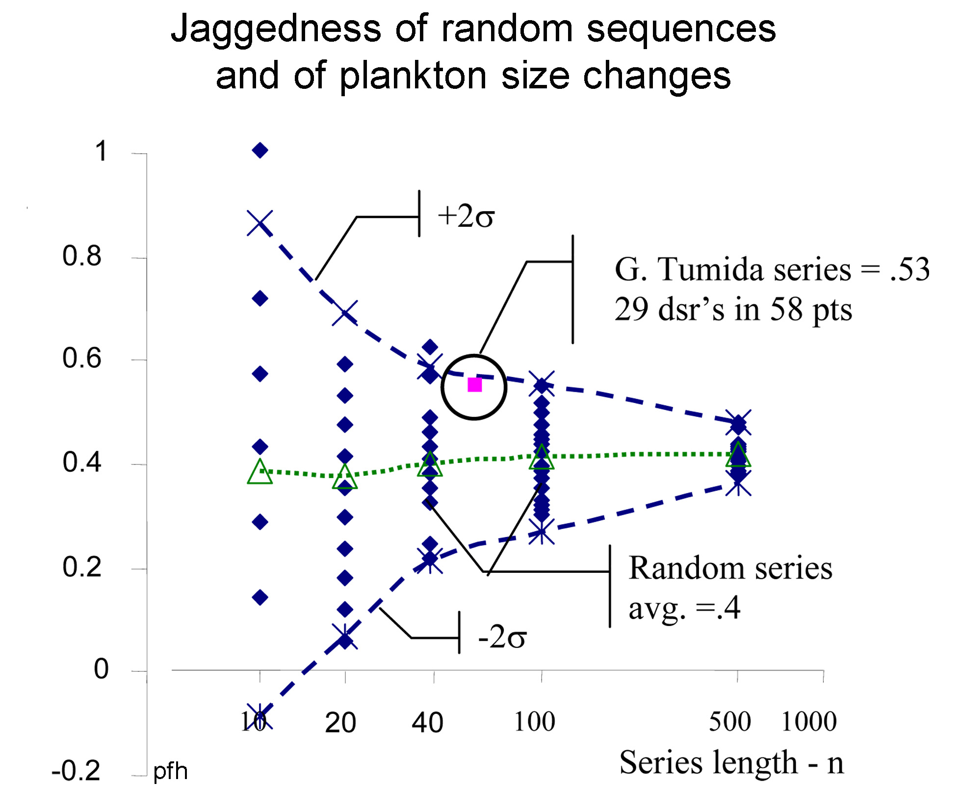
As compared to random variation, the test shows whether light smoothing quickly reduces the jaggedness of a series (the frequency of double reversals of direction). That would indicate a likelihood of there being flowing shape in the larger scale variations, and therefore also dynamic system processes producing the larger shapes. It remains to study the context to see if the implied shapes found can be confirmed.
|
|
|
|
1. Fraction of Double Slope Reversals (Jaggedness) - for random series compared to sequence of G. tumida sizes; using 20 random series of 10, 20, 40 & 100 point lengths, showing the mean jaggedness and 2 std. deviations above and below, and for the 58 point G. tumida data. |
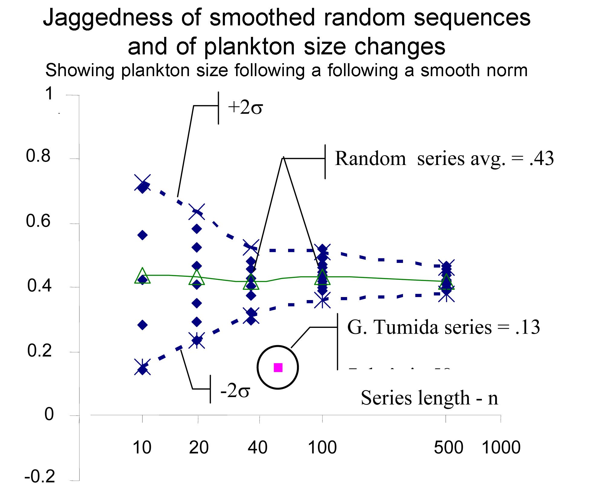
2. Smoothing Sensitivity - for same random series and G. tumida data, light smoothing does not change the scale of jaggedness for random series data, and does for the G. tumida data. Jaggedness of .13 for is well beyond 2s below the mean for the random series. Smoothing done by a 3 point centered kernel (1,2,1). |
The Case of G. tumida
) |
For the case of punctuated equilibrium in a plankton species for which
this test was developed the rather strong appearance of repeated
developmental spurts and dips in the rate of species size changes, revealed
as along smooth paths by light smoothing, was considered sufficient basis to
think through the implications and the other sources of evidence that might
confirm such a finding. Were the large shapes here part of a noise fluctuation rather than process fluctuation, the jaggedness of the curve would have been reduce a much smaller amount. You can clearly see the long strings of points with no point-to-point double reversals in direction [/\/]. It appears to indicate the underlying process is continuous rather than statistical This was the critical test for raising the question of whether the G. tumida data shows repeated evolutionary spurts and falls during the half million year progression from one form of the plankton to another for full discussion see 2007 Speciation of G. pleisotumida to G. tumida |