(excerpt from 5/98 version of " Modeling Evolutionary Rates With Proportional Walks; The Globorotalia Tumida Lineage Revisited". (c) P. Henshaw)

Once there is justification for assuming that a sequence of points reflects continuous processes of some scale there is a valid basis for attempting to reconstruct the behavior by curve fitting with functions or iterative methods like derivative reconstruction. To validate any results it remains, of course, to correlate the discovered behavior with theory and independent evidence.

It usually appears that there is also a random noise component present in any sequence of measures. In the design of derivative reconstruction it is presumed that this is illusory, that the appearance of random noise is generally evidence of continuous processes of great complexity or short duration that are poorly described, and not random behavior. Processes represented only by single points, for example, are naturally not reconstructable. It is therefore helpful to determine what scales of variation in the data reflect only short duration processes and what scales reflect complex superposition of longer duration processes. If it is possible to suppress the data reflecting processes of shorter duration than the sampling rate, without altering complex information about longer duration processes then the resolution of those complex processes can be improved.

When complexity in the data is a result of sampling from multiple scales of continuous fluctuation derivative reconstruction can often isolate each one separately. In one study (Henshaw notes 1997a) three smooth rates of oscillation were superimposed and then loosely sampled to create test data with an appearance of highly erratic fluctuation. Derivative reconstruction was quite effective in recreating the composite curve and then separating the original components. Any kind of noise suppression applied to the test data in that case would have destroyed all of the subtle evidence of derivative progression and made the reconstruction of the components completely impossible.

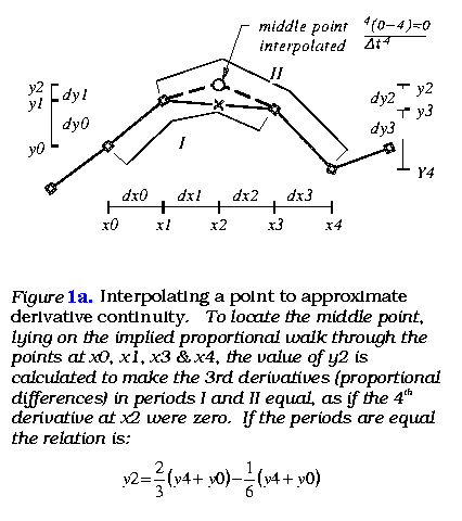
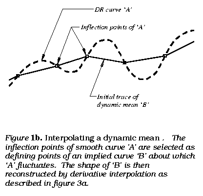
The first step is to interpolate a regular curve between the data points, following every wiggle, by inserting points resulting in the smoothest progression of rates of change possible. This concerns how the assumed or implied continuity would progress between points and is done with derivative interpolation. The present algorithm inserts a point where successive third sequential differences (derivatives) are equal (figure 1a). The second step is to construct that curve's dynamic mean, a smooth curve threading through the smallest scale fluctuations, as if the smallest scale of fluctuation were an elastic oscillation about a dynamically changing norm. This can be called integral interpolation and concerns the accumulative effect of the smaller fluctuations. The present technique does this by constructing a curve passing through the inflection (curvature reversal) points of the first. These two steps are repeated and result in a kind of 'smoothing', by separating the larger and smaller scales of variation.

The key analytical routine calculates the location of a point according to the rates of change implied by the two points before and after it, by equating the adjacent third sequential differences (3^rd derivatives). For the case of equally spaced points the value of the new point as given in equation (10) and illustrated in figure 1a.

y₂ = 1/3(y₁ + y₃) + 1/6(y₀+y₄) (10)

This relation is arrived at by first taking the successive differences:

The point 'O' in figure 1a is the result given by the 3^rd derivative interpolation. The point 'X' is the point that would result from linear (0^th derivative) interpolation. Linear interpolation is valid only when the rates of change approaching and following the point are the same. Using 4^th or higher derivative interpolation would follow the same scheme, though they have not been tested.

Partly because this algorithm is an imperfect approximation, and partly because of fine scale irregularity present in most data sets the same routine is often re-run, sequentially adjusting, rather than inserting, the points of the sequence to produce derivative regularization. This reduces fluctuation in the higher derivatives with limited effect on the path of the curve. It does slightly degrade the original information content and is used with discretion. Repeated derivative interpolation and regularization produces a differentiable curve in the limit, a proportional walk.

When used to successively adjust points for derivative regularization each point directly contributes to determining adjusted locations for two preceding and two following points. The original value of any point is not considered in determining its own adjusted value, except in so far as it has effected the locations of preceding points. A directional bias that arises is compensated for by separately scanning the sequence forward and back and averaging. After a few iterations little further alteration of the shape of the curve is possible as only its smoothness is effected.

The derivatives (plots of the sequential differences) of a proportional walk display the progression of rates of change implied by the data in great detail. In particular, they precisely locate the implied inflection points of the smaller scale fluctuations and allow an accurate reconstruction of the dynamic mean of the first curve, representing a larger scale process underlying the smaller scale fluctuations. This is illustrated in figure 1b. Integral interpolation isolates the scales of regular behavior and allows them to be independently studied. A variety of experimental studies demonstrate that this can be quite effective in depicting fine scale details of the larger scale processes. Findings include high degrees of synchrony between turning points for second and third level dynamic means for behaviorally linked measures such as earth temperature and atmospheric CO₂ and aggregate economic indicators, that were not at all apparent in the data(Henshaw notes 1997c). The studies also demonstrate some of the limitations of the method.