Reconstructing a sampled composite function (full size)

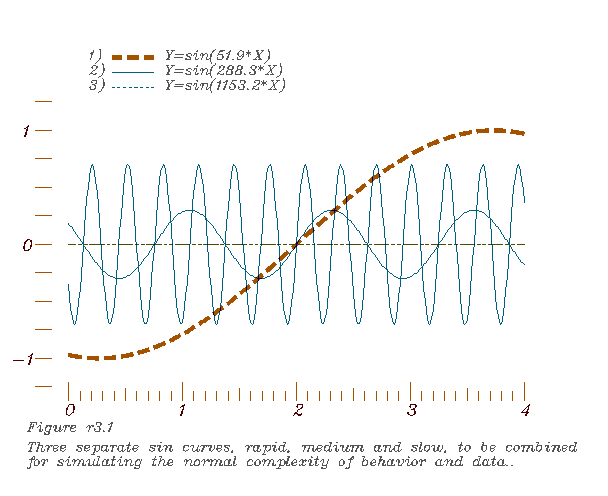
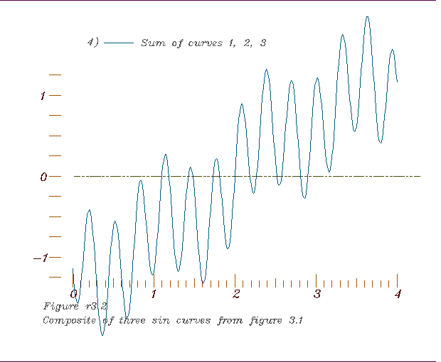
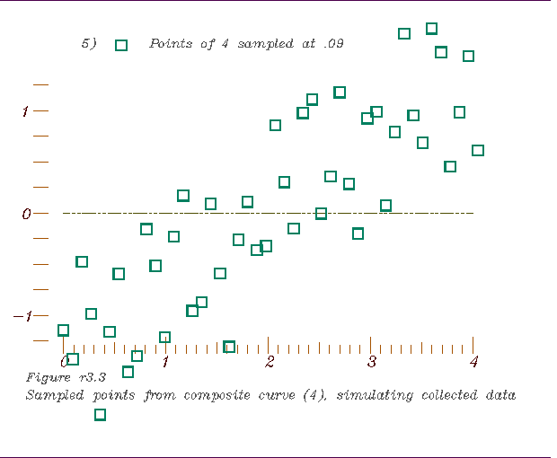
To test the DR method a sin curve is 'disguised' by superimposing two other sin curves of higher frequency and then sampling values from the composite to see if the components can then be reconstructed.

Normal curve fitting methods would treat the data produced this way as statistically distributed around a single function, probably producing a straight line and a random variable. A keen observer would note the cyclic pattern in the data and might separate these very regular components. DR works just as well when the data is real, with irregular, asymmetric and transient underlying processes to be separated out.

The figures display the compound sin curve test procedure in12 steps:
(open two browsers to view figures side-by-side)

1. Selecting three regular mathematical functions,

2. The composite to be sampled

• 3. A periodic sampling of points to simulate a data set representing a complex of processes.

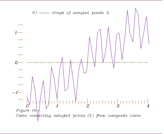
4. A graph of the selected points,

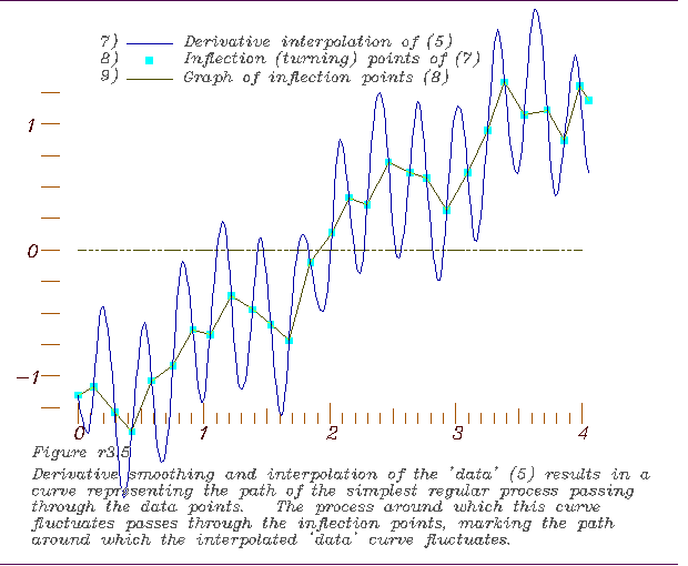
5. Derivative interpolation of the data and location of its inflection points,

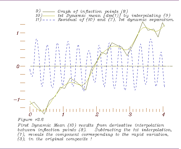
6. Derivative interpolation of those inflection points to form the 1st dynamic mean,

7. Inflection points of the 1st dynamic mean,

8. Derivative interpolation based on inflection points of 1st dynamic mean to form the 2nd,

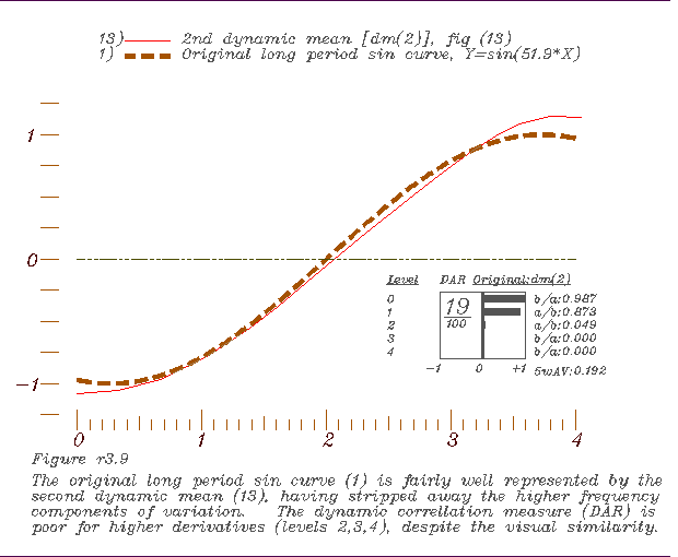
9. Comparing the 2nd dynamic mean with the long period sine curve.

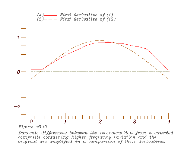
10. Comparing the 1st derivatives of the 2nd dynamic mean and the long period sin curve,

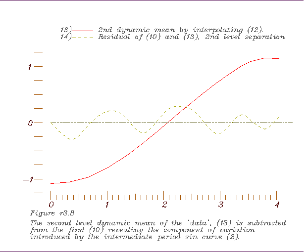
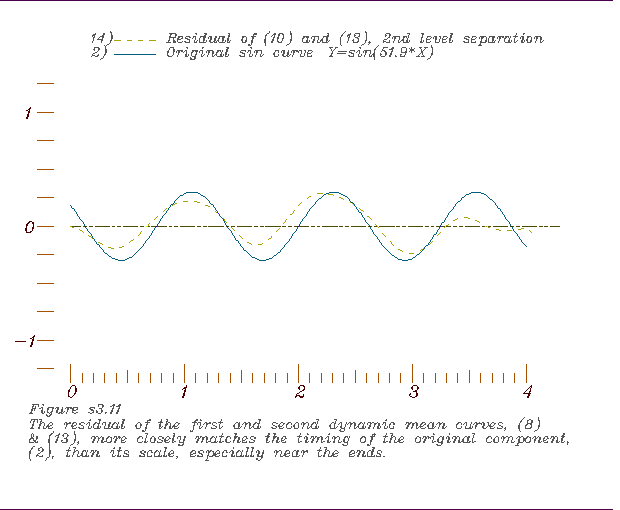
11. Comparing the residual of the 2nd dynamic mean and the 1st with the medium period sin curve,

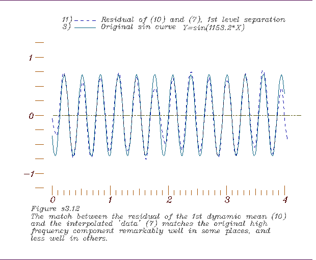
12. Comparing the residual of the 1st dynamic mean and the short period sin curve

back to the DR main page